System model
I built a simulation of a two-axis robotic tracking platform and a moving target. The model joins the platform's azimuth and zenith axes, stepper-driven servo dynamics, target motion, camera bearings and a range sensor. The estimator's job is to turn these asynchronous, noisy measurements into a time-aligned target position and velocity for the tracking controller.
Frames and spherical coordinates
The target is represented relative to the platform base by range r, azimuth θ and zenith φ. With zenith measured from the vertical, its Cartesian position is:
x = r sin(φ) cos(θ)
y = r sin(φ) sin(θ)
z = r cos(φ)
The corresponding velocity separates naturally into radial and angular motion:
v = ṙ er + r sin(φ) θ̇ eθ + r φ̇ eφ
The angular-rate terms are scaled by range; azimuth rate is also scaled by sin(φ).
Stepper-servo and platform dynamics
Rather than treating a stepper as an ideal position source, I modelled its discrete stepping, friction and actuator response. That gives the simulated tracking loop a more realistic plant for checking the position response. The two platform axes are represented by angle/rate states, with motor torque driving angular acceleration:
Jθ θ̈ = τθ
Jφ φ̈ = τφ
Each encoder observes angle directly, while angular velocity is estimated. For either axis, torque and moment of inertia define the angle/rate state model:
xa = [α, α̇]T
ẋa = [α̇, τa/Ja]T
ya = [1, 0] xa + v
The range filter uses a constant-acceleration state, with range as its measured output:
xr,k = [r, ṙ, r̈]T
xr,k+1 = [[1, Δt, Δt2/2], [0, 1, Δt], [0, 0, 1]] xr,k
zr = [1, 0, 0] xr + vr
The stepper-servo simulation supplies the actuator response used by the tracking model.
Friction, compliance and cogging
The actuator model includes rotor and load inertia, the stepper's magnetic spring, drivetrain compliance, damping, and static and dynamic friction. I tuned the spring, damping and friction gains against measured small-step encoder responses so the model reproduces the drivetrain's oscillation and load lag, rather than assuming a rigid, frictionless axis.
Detent (cogging) torque repeats with rotor electrical angle. I characterized the periodic angle error in slow rotations in both directions and used its repeatable component to build a zero-mean lookup-table correction. This feed-forward compensation targets the periodic error without treating it as random sensor noise.
Hardware setup
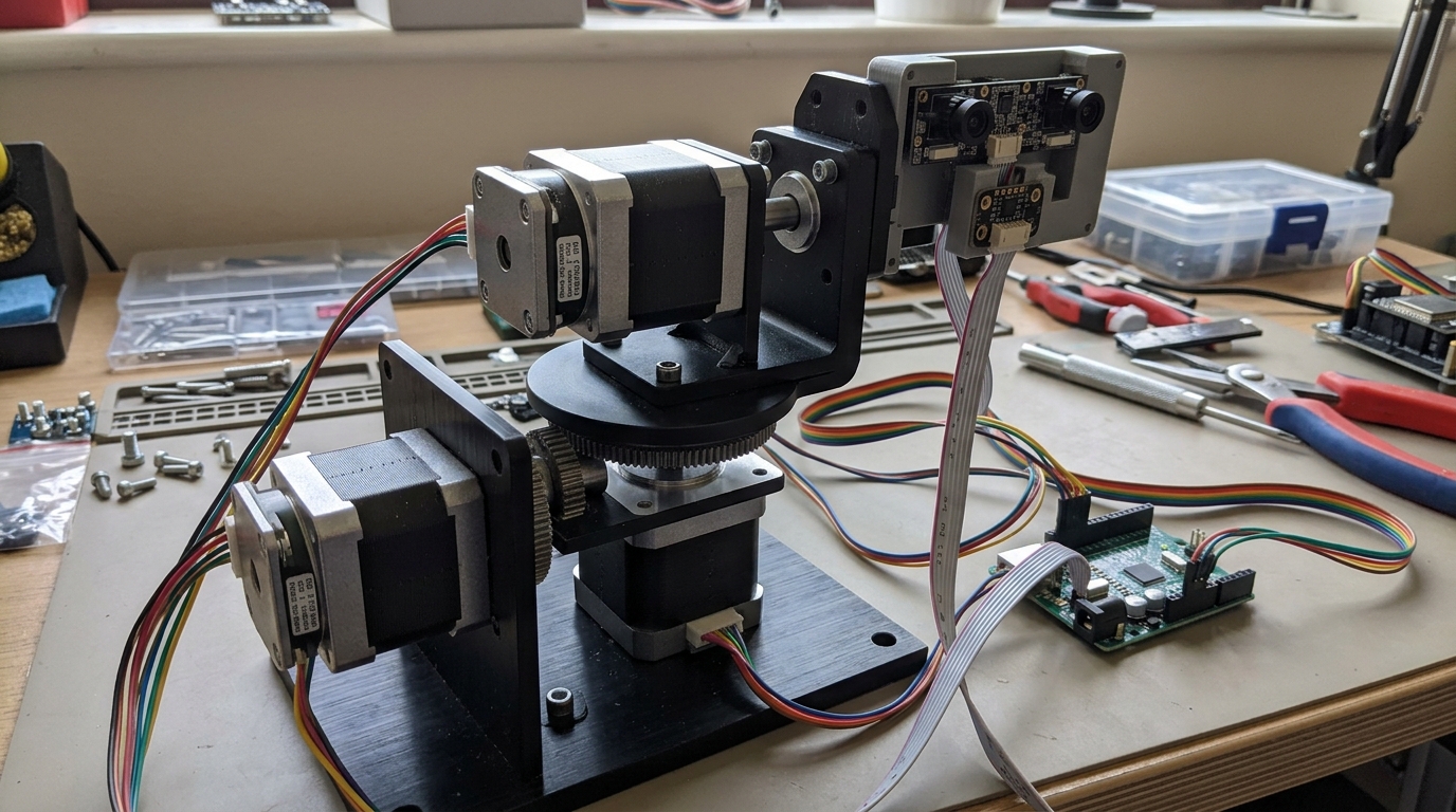
The bench prototype pairs the two-axis mechanism and its sensors with an STM32H7 controller. The diagram shows the functional signal and power paths; exact pin assignments, bus protocols and supply voltages are not specified here.

Target-motion model
The EKF tracks a nine-element state in the base frame, including range, azimuth and zenith, their rates, and three slowly varying acceleration-disturbance terms:
x = [r, ṙ, θ, θ̇, φ, φ̇, ar, aθ, aφ]T
The base model holds the acceleration-disturbance states between updates: ȧr = ȧθ = ȧφ = 0.
In spherical coordinates, the nonlinear motion equations couple range and angular motion. The centripetal terms matter: angular velocity changes the radial acceleration, while range and zenith motion affect azimuth acceleration.
r̈ = r φ̇2 + r sin2(φ) θ̇2 + ar
θ̈ = -2 θ̇ (ṙ/r + cot(φ) φ̇) + aθ/(r sin(φ))
φ̈ = sin(φ) cos(φ) θ̇2 - 2 ṙ φ̇/r + aφ/r
Measurement fusion and the EKF
The range sensor measures r; the camera measures target azimuth and zenith relative to the moving platform. I transform those camera bearings into the base frame using the measured platform angles before updating the target filter. In compact form, the sensor vector is z = [r, θcam, φcam]T, with the bearing components mapped into the base-frame observation model.
pB = Rz(θa) Ry(φa) Rz(θcam) Ry(φcam) [0, 0, r]T
The rotation chain maps the measured camera ray through the moving axes into the fixed base frame.
The platform angle and range filters are linear KFs; the coupled target model is nonlinear, so its EKF linearizes the motion and measurement functions at each predicted state:
x̂-k = f(x̂k-1, uk-1)
P-k = Fk Pk-1 FkT + Q
Kk = P-k HkT (Hk P-k HkT + R)-1
x̂k = x̂-k + Kk [zk - h(x̂-k)]
Pk = (I - Kk Hk) P-k
STM32H7 controller and asynchronous timing
The STM32H7 is the real-time control target. The two axis encoders and their linear Kalman filters run on a 2 ms step, range readings arrive asynchronously at up to 20 Hz, and camera updates arrive at 60 Hz with about 16.6 ms of latency. Before the target EKF update, the encoder estimates are interpolated to the camera timestamp and the camera bearing is transformed into the platform base frame.
The EKF provides the controller with the estimated target position and velocity. Because a camera observation is already about 16.6 ms old when it arrives, the state is advanced to the STM32H7 controller's next 100 μs (10 kHz) tick using Tustin (trapezoidal) integration:
x(t + Δt) ≈ x(t) + (Δt/2) [ẋ(t) + ẋ(t + Δt)]
This compensates for camera age and produces a current target state for the fast tracking loop.
For tracking, each axis uses proportional feedback with a feed-forward term (P + FF). For point-to-point A-to-B moves, the platform uses a PI controller. The EKF supplies a time-aligned target state for tracking, while the actuator model captures friction, drivetrain compliance and cogging effects.
Selected results
These results are specific to their test conditions and are not a general accuracy guarantee. The measured outcomes below are not a direct controller-to-controller comparison.
| Test | Result | Conditions / interpretation |
|---|---|---|
| A-to-B positioning | Within ±1 arcsec (about ±4.85 µrad) in 2.7 s | Higher-inertia azimuth axis; achieved in both directions on the tested setup. |
| Cogging compensation | Azimuth RMS tracking error: 53 → 27 µrad | 85 s hand-trajectory test, comparing compensation off versus on. |
| Simulation vs. hardware tracking | Qualitatively similar behaviour | A hand-trajectory segment; not a quantitative precision validation. |
Model predictive control (MPC)
MPC uses a dynamic model to predict the platform's motion and optimizes a sequence of control actions at each update, subject to actuator constraints. It applies the first action, then replans from the latest state estimate. This makes it possible to tune the balance between tracking accuracy and control effort while explicitly limiting motor speed and torque.
For this platform, the linear MPC was configured to stay within a linear motor operating region and avoid transmission slip. Its weights, control and prediction horizons, and optimizer iteration limit can be tuned; the A-to-B setup used five control-horizon blocks and up to three iterations. MPC requires a state estimate, and capturing gearbox oscillations adds complexity to the model and estimator.
MPC compared with the selected controllers
The P + feed-forward tracking controller is computationally light, while the PI controller handles A-to-B positioning. In A-to-B simulation, the linear MPC with the OneStep state estimator met the <1 arcsecond precision requirement. This was not a same-condition comparison against the selected PI controller, so it does not establish a direct accuracy improvement.
| Measure | Selected control | Linear MPC |
|---|---|---|
| Application | P + feed-forward for tracking; PI for A-to-B positioning. | Evaluated for tracking and A-to-B motion; more tuning options and explicit speed/torque limits. The simulated A-to-B move met <1 arcsecond precision. |
| Computation | Lower computation for the selected controllers. | Up to 300 µs for tracking in the benchmark (about 125 µs per axis when scaled to a 480 MHz H7); about 175 µs per axis for A-to-B with reference preview. |
| Final choice | P + feed-forward was chosen for tracking and PI for A-to-B moves; MPC was not selected because of its higher computational cost. | |